A research communication project by Niklas Schmid, André Warnecke and Prof. John Lygeros.
The Ball-on-Plate System
The Ball-on-Plate is the 90’s Arcade experience re-imagined.
The Ball-on-Plate (BoP) system is an interactive demonstrator to explain automatic control to the general public.
It was developed by Niklas Schmid, André Warnecke and Prof. John Lygeros in 2026 at the Automatic Control Laboratory at ETH Zurich.
We currently have three prototypes, each with its own purpose and design:
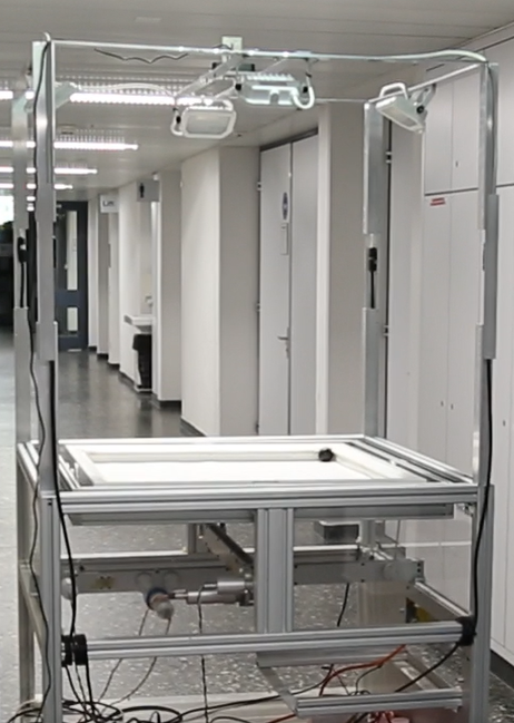
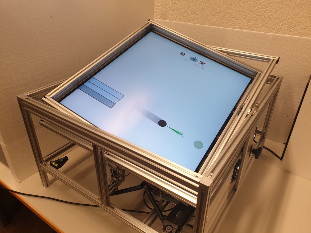
BoP Senior: Exhaustive research experiments.
BoP Junior: Public exhibitions.
BoP Mini: Small desktop version for teaching in schools. (In development, expected release in 2027.)
BoP SeniorBoP Junior
What is Automation?
Automation consists of the use of technology to perform tasks without or with minimal human intervention.
Dynamical systems, like the BoP exhibit, are made up of mechanical and electrical components (such as motors and sensors, such as cameras) that are interconnected and governed by software. The software uses algorithms to command the components based on sensor measurements to achieve a desired behavior (such as keeping the ball in the center of the plate).
Control theory is the mathematical study of designing such algorithms to automate systems.
How does Automation work?
How can algorithms fly airplanes and drive cars autonomously?
We can use the BoP exhibit to understand how automation works.
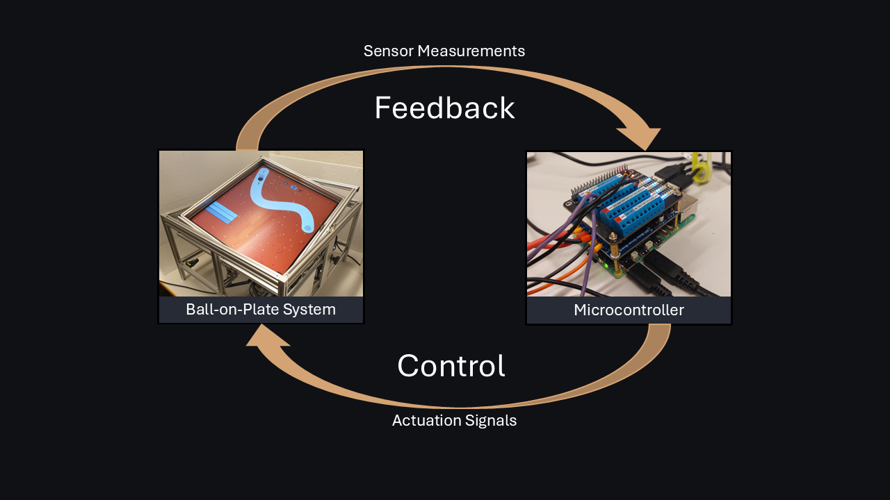
Assume we want to direct the ball to the center of the screen. Sensors measure the ball position. The data is sent to a microcomputer (feedback), which computes tilt angles for the plate. The tilt angles are chosen such that the ball moves towards the plate's center, and achieved by sending respective voltages to the motors (control). This process is repeated over and over again, leading to a feedback loop that continuously corrects the ball's position towards the center.
Figure 1: Feedback loop in control systems.
But how does the computer know which plate angles move the ball towards the center? There are lots of different methods of control that can be used, and here we will look at seven of them:
Linear Feedback Control
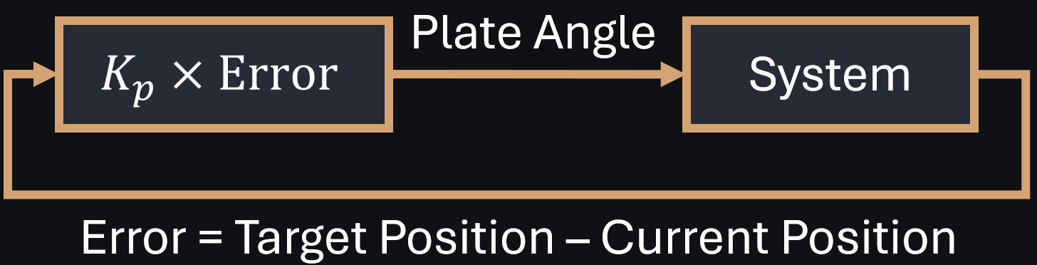
Imagine holding the plate in your hands. If the ball is to the left of the center, you will tilt the plate to the right, and vice versa. The further away the ball is from the center, the steeper you will tilt the plate. Linear feedback controllers do precisely that: They take the difference of the ball-position from the center and multiply it with a constant (Kp). The product is the plate angle, which is achieved by outputting a respective voltage to the motors.
Figure 2: Linear Feedback Controller with gain Kp.
If the gain is chosen well, the ball automatically moves to any desired position on the plate. However, there is room for improving performance!
The controller uses the green circles as reference. The controller has three parameters (Q_pos, Q_vel, R) that are used to weight three tuning-objectives: The controller must reduce the distance between the ball's position and the targets to reach the targets (weighted by Q_pos), the controller must maintain a small velocity on the ball to prevent the ball from bouncing around wildly (weighted by Q_vel), and the plate angle shall remain small to prevent the plate from shaking back and forth aggressively (weighted by R). Weighted by these parameters, we compute a feedback gain Kp that finds a good trade-off between our tuning-objectives. Increasing Q_pos, and decreasing Q_vel and R makes the controller more aggressive, i.e., Kp gets larger. The video shows how the control behavior changes as we adapt the parameters online (bottom left). Animation designed by David Lammering.
Proportional-Integral-Derivative Control
When the ball is standing still, static friction causes the ball to stick even if the plate is slightly tilted. This friction can greatly affect control performance: Recall that a linear controller multiplies the difference between the ball and target position with a constant number to compute the tilt angle. If this factor is too small, the ball may never start rolling. As a human, we would carefully increase the tilt angle incrementally until the ball begins to roll. In control theory, this is called integral control: The algorithm sums the difference between the ball's current and desired position, multiplies this sum by a factor, and sets the plate's tilt angle to the resulting product. As long as the ball does not move towards the target, e.g., due to static friction, integral controllers keep increasing the tilt angle.
Once the ball starts rolling, humans typically try to counter this movement to reduce velocity and avoid overshooting the target. This is mimicked by acting against the change of error, i.e., we multiply the change of the error by a constant factor and set the tilt angle to the resulting product.
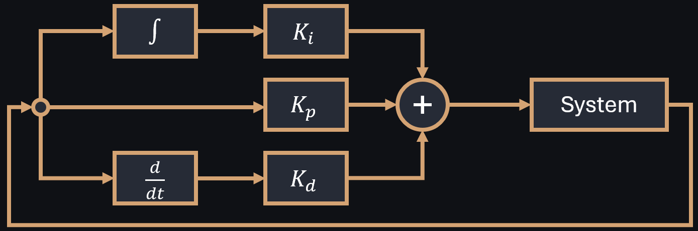
None of these controllers works well just by itself. Instead, all have their own strengths and weaknesses. To combine these strengths, a common approach is to just use them all at the same time, and sum their signals, leading to so-called Proportional-Integral-Derivative-controllers (PID).
Figure 3: PID Feedback loop in control systems.
Sounds too simple? In fact, such controllers are the de facto industry standard for simple automation tasks, and more than sufficient to balance the ball of our system in the center:
Flappy-ball - Our interpretation of the popular mobile game. We use a PID controller to keep the horizontal position of the ball constant, and another PID controller for the vertical axis to move the ball to the height of the upcoming gate. The colored area behind the ball symbolized the summed error to the reference. The individual P-, I-, and D-outputs and their sum (the requested plate angle) are shown via bar plots on the right. Animation designed by David Lammering.
Check out portafilter machines at you local coffee machine store. Some particularly expensive machines advertise their fancy "PID temperature control". This means that there is a built-in temperature sensor, and a small computer that increases or decreases heating using a PID controller until a desired temperature is reached. Not really high-tech (particularly given the price of these machines) but it does the job!
Similarly, we could implement PID controllers to program an airplane's autopilot. If the airplane looses altitude, the PID controller adjusts the elevators on the tail to manage the airplane's pitch and maintain a set altitude. This ensures that any deviations caused by turbulence or air pressure changes are corrected smoothly.
Model Predictive Control
PID controllers are intuitive and simple to implement, but they have their limitations. A simple example where PID controllers are often insufficient is in the face of safety critical constraints of operation (e.g., a car must not crash into a wall). Imposing such operational constraints via PIDs requires careful tuning and thorough validation, which is time-consuming and error-prone. It is also possible to damage your system while trying to find safe gains for your PID controller.
Humans enforce safety by anticipating the consequences of their actions, and correcting their behavior before getting close to a dangerous state. For example, when driving a car, we will slow down before a sharp turn. Model Predictive Control (MPC) mimics this philosophy. The idea is to predict the system evolution under a control signal for a few seconds into the future using a mathematical model of the system. The computer then crunches numbers to find control signals that are safe and yield good performance.
The animation shows the optimized predicted trajectory of the ball. The optimization is updated frequently to update the ball's predicted position based on latest measurements.
The video shows the optimized predicted trajectory of the ball. The trajectory is reoptimized whenever a new measurement of the ball's position is available. Animation designed by Samuel Baumgartner and Florian Borchard.
Model Predictive Path Integral Control
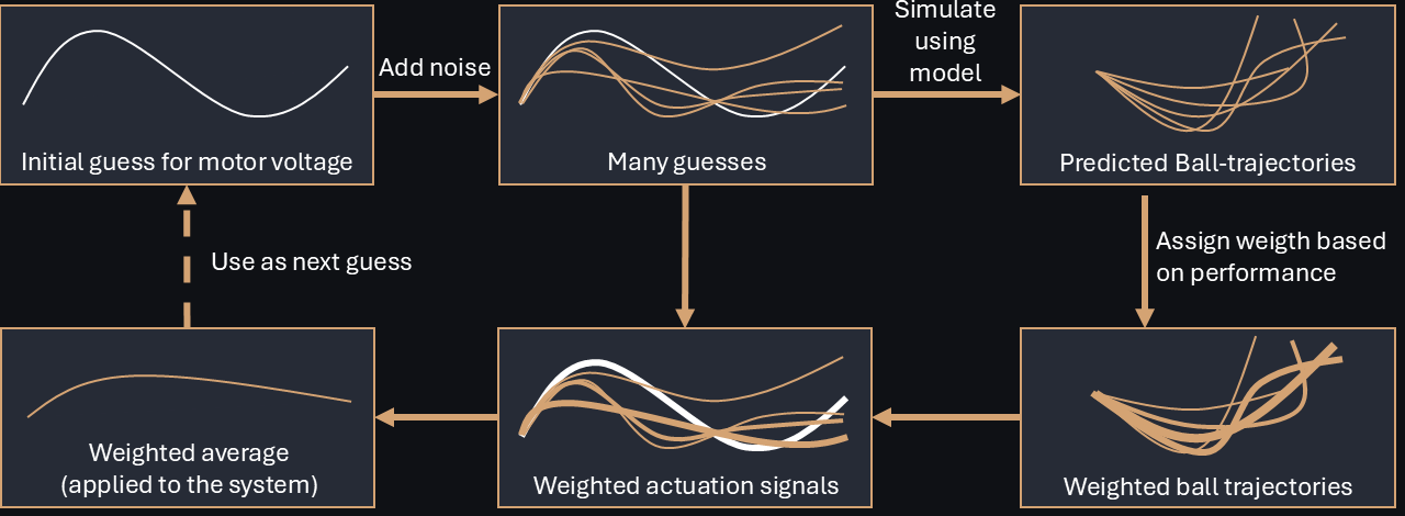
Model Predictive Control works well on very specific types of systems, but can fall short when those systems become more complex. For instance, it cannot model collisions from the boundary of the plate and use bounces off the wall as part of the ball's trajectory to collect points faster. A (somewhat brute force) alternative for optimizing input signals with predictions is Model Predictive Path Integral Control (MPPI). We start with some initial input sequence, copy it a thousand times, randomly modify each copy slightly to obtain many diverse but similar input sequences, and compute a weighted average based on the resulting performance of each perturbed signal. This approach is rather new, enabled by the abundance of computational resources. It is particularly popular for robotics systems such as humanoids and quadrupeds since it can model arbitrary complex dynamics and physical constraints.
Figure 4: Model Predictive Path Integral Control.
The animation shows the many samples used to find an optimal trajectory for the ball. Similar to MPC, the prediction is regularly updated based on the ball's position.
The animation shows some of the ball trajectories predicted by the MPPI controller (it actually generates a thousand every few milliseconds!). The algorithm evaluates every trajectory, gives them a high or low weight depending on how close they bring the ball to the targets, and then executes a weighted average trajectory. Or at least, it executes the first bit of every trajectory: Similar to MPC, the trajectory is replanned every time there is a new measurement of the ball position. Animation designed by Samuel Baumgartner and Florian Borchard.
Rapidly Exploring Random Trees
MPC and MPPI only plan optimal input sequences over a limited prediction horizon, which makes them less effective for planning long-term paths. For instance, if a goal is placed far from the current position, these methods may struggle to find a viable path.
In contrast, path planning algorithms keep search for complete paths that reach from the current state to the target, no matter how long it takes to compute this path. Rapidly Exploring Random Trees (RRT) are one such type of path planning algorithms. RRT starts at a random point in space and sprouts new branches from it toward other random points in space, progressively expanding until one of these branches reaches the target. This is similar to drawing lines with a pen in a maze until you find a path to the exit.
Such algorithms are particularly useful for navigating in complex environments with obstacles, e.g., for humanoids in buildings.
The animation shows the generation of such a tree. Once a path is found by RRT, any of the previously discussed controllers may be used to get the ball to actually follow it.
For computational reasons, MPPI can only look a few seconds into the future. This can make it difficult to find paths around obstacles and lead to suboptimal performance. In contrast, RRT aims to find complete paths from the starting state to the target. This path can then be tracked using, e.g., MPPI. Therefore, RRT constructs a which rapidly grows around obstacles until it hits the target (red cross). Animation designed by Louis Miller.RRT can find paths through complex environments. Animation designed by Louis Miller.
Dynamic Programming
Usually one aims to find the path that is shortest, fastest, or most energy efficient. RRT does not guarantee any of that, neither does it ensure that the system is actually able to track the path. Dynamic programming algorithms address this limitation.
A bit mind-twisting: The algorithms starts at a future point in time, and then iteratively decides backwards in time on the best input from every state. More specifically, at every time-step, the algorithm assigns a cost-value to every state. If the target is easy to reach from a given state, or if states with low cost-values are within reach, the algorithm assigns a low cost-value to this given state. If it is hard to reach the target or states with low cost-values, a high cost-value is assigned to that state. Once the value of all states is known, any previously discussed controller can be used to move the ball towards states with low cost-values, guiding it to the target.
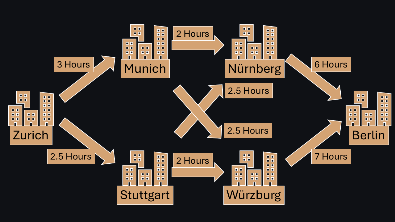
We use similar intuitions everyday: Imagine you are trying to travel from Zurich to Berlin. Dynamic Programming would search for the optimal path starting from Berlin. The cost-value of a city is the minimum time it takes to travel to Berlin. Nürnberg to Berlin takes 6 hours, so a cost-value of 6 is assigned to Nürnberg. Würzburg to Berlin takes 7 hours, so cost-value of 7 is assigned to Würzburg. Munich to Würzburg takes 2.5 hours (leading to a total of 9.5 hours to Berlin), but Munich to Nürnberg takes only 2 hours (leading to a total of 8 hours to Berlin). Dynamic Programming chooses the least-cost option leading to a cost-value of 8 for Munich. Continuing this process for Stuttgart and Zurich leads to the optimal path from Zurich to Berlin via Munich and Nürnberg, with a total cost-value of 11 hours. In fact, these simple principles are used in apps like Google Maps and Waze (just highly optimized).
Figure 5: Finding the fastest way from Zurich to Berlin via Dynamic Programming.
We use Dynamic Programming to navigate our ball through obstacles towards a target region. Once the value of all states is known, any previously discussed controller can be used to move the ball towards states with low cost-values, guiding it to the target. The animation shows the cost-values assigned to each state as a heatmap that is computed backwards in time, and the controllers' targeted ball position as green circles once all cost-values are computed.
The ball navigating through obstacles (red) using Dynamic Programming. The heatmap shows the cost-values assigned to each state. Orange indicates low values, and green indicates high values. The circles represent the targeted ball state, which is always towards high values. Animation designed by Oliver Baumgartner.
You could also think of using Dynamic Programming for autonomous driving. The algorithm would assign low cost-values to states that are close to the desired destination and far from obstacles, and high cost-values to states that are far from the destination or close to obstacles. The car would then use a controller to steer towards states with low cost-values, effectively navigating towards the destination while avoiding obstacles.
Reinforcement Learning
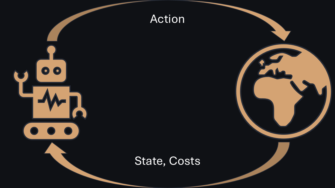
Dynamic programming is a powerful tool for planning paths optimally, but it requires a perfect model of the system. Many real-world applications are subject to complex dynamics, where models are not readily available (e.g., robots with hundreds of motors and joints). Reinforcement learning (RL) mimics human learning through trial and error. Similar to Dynamic Programming, if a state led to a good outcome, it is assigned a low cost-value. It is assigned a high cost-value otherwise. The outcomes of every action from every state is memorized using a neural network. Simultanously, another neural network is trained to output plate angles that move the ball towards states with low cost-values.
Figure 6: Reinforcement Learning controllers don't use a model, but learn to minimize costs by interacting with the world through trial and error.
The animation shows the activity of the neural network based on the current ball and desired target position.
The ball is manouvred through obstacles using Reinforcement Learning. The graphic shows the neural network's activity based on the current ball and desired target position (green circles). Animation designed by Oliver Baumgartner.
BoP Research
We use the Ball-on-Plate system to benchmark the performance of our researched control algorithms. Several publications are in the making and will soon be explained visually here!
BoP Education
Systems are often complex, which renders controller design challenging. If a quadcopter crashes, it is often hard to say what went wrong. The controller could have been too aggressive, too mild, too slow, or just turn on completely wrong motors - the quadcopter quickly crashes in either case. In contrast, the Ball-on-Plate system has two benefits: First, the dynamics are rather slow, which makes it easy to visually analyse how the controller behaves. Second, it is intuitive what a "good" control behavior should look like: If the controller is computed too slowly, then the plate angle changes directions with a notable delay; if the controller is too aggressive, then the ball overshoots the target; if the controller is too mild, then the ball gets stuck before reaching its target due to static friction; if there is a sign error in the controller, the plate tilts in the wrong direction. This way, bad control behaviors and bugs are easily identified and corrected. This makes the Ball-on-Plate system an excellent platform for teaching automation and for researching control algorithms. Taking this to the extreme, we are currently preparing a control workshop for 5th graders - more information coming soon!
Several thesis projects have already utilized the Ball-on-Plate system to develop and benchmark novel control approaches. Below is a list of current and past thesis projects:
Name
Title
Year
Supervisors
Oliver Baumgartner, Samuel Baumgartner, Louis Miller, David Lammering, Florian Borchard
Interactive Control Research Communication using the Ball-on-Plate system
2025
Niklas Schmid, André Warnecke
Salma Elfeki
High-Performance MPC Controllers Under Environmental Changes
2025
Niklas Schmid, Riccardo Zuliani
Jonathan Hilberg
Model Free Joint Chance Constrained Optimal Control
2024
Niklas Schmid, Marta Fochesato
Alexander Kaspar
Meta-Learning Model Predictive Control for the Ball-On-A-Plate System
2024
Niklas Schmid, Jiaqi Yan, Riccardo Zuliani
Mirco Vandeventer
Meta-Learning Reinforcement Learning for the Ball-On-A-Plate System
2024
Niklas Schmid, Jiaqi Yan
Simon Frölich
Hardware Reconfiguration and Control of the Ball-On-A-Plate System
2024
Niklas Schmid
Elias Bai
Improved Reinforcement Learning Control of the Ball-On-A-Plate System
2023
Niklas Schmid
Joram Ebinger
LQR and Reinforcement Learning Control of a Ball-On-A-Plate System
2023
Niklas Schmid
Acknowledgement
The Ball-on-Plate system is designed by Niklas Schmid,
André Warnecke and
Prof. John Lygeros
at the Automatic Control Laboratory, Department of Information Technology and Electrical Engineering, ETH Zurich.
The BoP Senior system is based on a prototype constructed by Olaf Hermann in 1997.
The project is financed by the Swiss National Science Foundation under NCCR Automation under grant 51NF40_225155.
We further thank all students who contributed to this project.
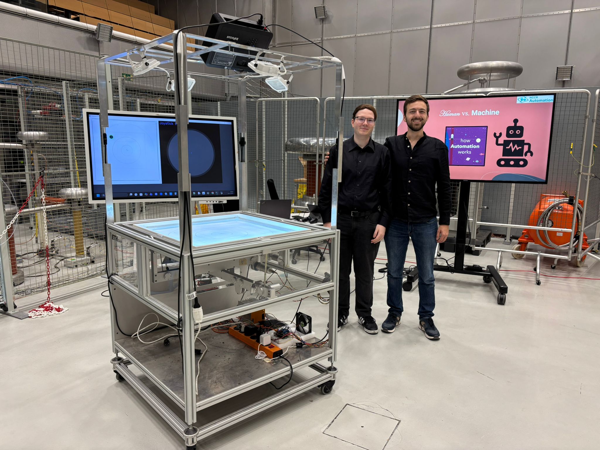
Figure 7: André Warnecke (left) and Niklas Schmid (right) presenting the Ball-on-Plate system.
For any questions, suggestions, or ideas for collaboration, please reach out to us at
BoP@ethz.ch.